Why the Confusion Matrix Should be Called the Anti-Confusion Matrix
Whenever we are building a classification model we need to know good our model is at classifying the data we give it. A very basic way we can examine a model’s performance is by computing its accuracy. Unfortunately only looking at accuracy can give us the false idea that our model is performing well, when it isn’t. This is called the accuracy paradox.
Let’s look at an example to see what I mean. Say we want to predict which babies will be born with some rare disease based on a number of features we have reason to believe could help us make this prediction. We have a dataset with 1,000 babies that were born healthy and 100 that were born with the disease. We run our model and get 90% accuracy on our test set! We are happy our model performed so well and now we go to our colleagues and tell them that we have a model that can predict this disease with 90% accuracy. Except we’d be embarrassingly wrong.
What you have done is sorted babies into the correct categories, has disease and does not have disease, 90% of the time. In fact its very possible your model predicted that all babies did not have the disease to get an accuracy score of 90%. That’s the same as guessing!
This is why the confusion matrix is important to understand. It actually helps us prevent this kind of mistake. You might even say the confusion matrix is a tool to prevent confusion about the true performance of our classification model.
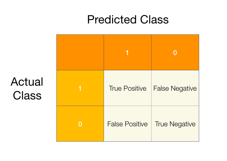
In a binary classification problem we pick one of the classes to be our positive class and assign it a value of 1. Then we label the remaining class the negative class and assign it a value of 0. When we run our model on our data there are two possible outcomes for each sample in our dataset, we can either predict it correctly, or we get it wrong. Since we have two classes there are two ways to get our predictions right and two ways to get it wrong as described in the confusion matrix below.

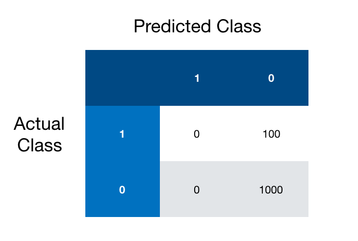
We call a prediction true when it is correct and false when it is not. Going back to our rare disease example we can fill in our confusion matrix with some made up data.

In the above we have set the positive class (1) to be babies who have the disease and the negative class (0) to be babies who don’t. Like I hinted at before the above confusion matrix shows how we could achieve a 90% accuracy score without correctly predicting any of the babies who have the disease.
While a 90% accuracy score might have seemed impressive, you or I could have done just as well by guessing that all babies don’t have the disease and calling it a day.
This should give us some intuition on why it’s important to understand the confusion matrix, and why it should be seen as a tool to prevent confusion and not a source of it. Next we will look deeper into how we can use the confusion matrix to learn about precision and recall.