Recently, I read an article where a current data scientist discussed her struggles to remember the difference between ridge and lasso regression.The goal of this post is to help those of you who are new to data science and are similarly struggling, hopefully get a better idea ridge and lasso regression.
Start With What You Know
Both ridge and lasso regression are ‘modifications’ of ordinary least squares linear regression. In OLS multiple linear regression our cost function is:
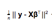
Here n is the number of data points or samples, y is our target vector, X is the input matrix, and β is our coefficients vector.
Question What You Know
OLS linear regression is a useful technique but its not always the ideal method. For instance, what about if we have outliers? Or how might multicollinearity affect our model? When asking questions like these it becomes clear that OLS is not always the idea method for regression.
Let’s say we want to run a linear regression on features that exhibit multicollinearity. Multicollinearity can cause our variance to be high, which will result in overfitting our model. Since we want our models to generalize to new data, it is helpful to have a method for preventing this kind of overfitting.
Regularization is a means to avoid high variance in our model. To do this we will introduce a penalty term to the cost function above. By adding this penalty term we will prevent the coefficients of the linear function from getting too large. Introducing this bias should decrease the variance and thus prevent overfitting.
The Ridge Cost Function
The ridge cost function adds the L2 norm of β as its penalty term, which is just a fancy way of saying we’re ‘adding all the coefficients squared’. This is not quite right because we want to have some control over how much the L2 norm of β will affect our model, so we multiple by a tuning parameter, λ.

When λ is significantly large the sum of squared errors term in our cost function becomes insignificant. Since we are looking to minimize the above function, this forces β to 0. So we see that as λ increases, the values in β decrease. This is the behavior we wanted, because it reduces the variance. You can just think about calculating the variance with smaller coefficients to see why this is the case.
The Lasso Cost Function
The lasso cost function on the other hand uses the L1 norm of β as its penalty term. The L1 norm of β is the sum of the absolute values of our coefficients.

Similarly as λ gets significantly large β is forced to 0. But what is important to note about the lasso cost function, is that because we are using the absolute value, instead of the square of our coefficients, less important features’ coefficients can be assigned a value of 0. This is particularly helpful for feature selection.
The reason why the penalty term results in coefficients being zero has to do with the constraint region, which I won’t go into here, but I recommend reading into because it will be helpful in order to cement the idea that the L1 penalty allows for some coefficients to be zero.

Putting it Together
Once we understand what ridge and lasso regression are doing, it is easier to remember which uses which regularization method.
Personally, I like to imagine a lasso pulling numbers down to zero on a number line. This reminds me that lasso regression can cause some of the model’s coefficients to be zero. Since the L1 norm creates the constraint region that makes this possible, we know that Lasso uses the L1 norm as its penalty term. If you remember that lasso and ridge use the L1 and L2 norms as penalty terms, it follows that ridge uses the L2 norm.
Hopefully this can help someone having a hard time keeping these two regression methods straight.