Gradient descent is a method that is commonly used in optimization problems. For instance if we want minimize the cost function of some model we might use gradient descent.
Two main reasons for using gradient descent:
- There is no easy way to get the derivative of our function or otherwise solve for the minimum.
- A way to solve for the minimum exists but it is too computationally costly as we increase the amount of data we use.
As an example, a well known method for finding the minimum of a linear regression model exists using linear algebra, but when we increase the number of columns and rows in our matrix it can be too computationally expensive.
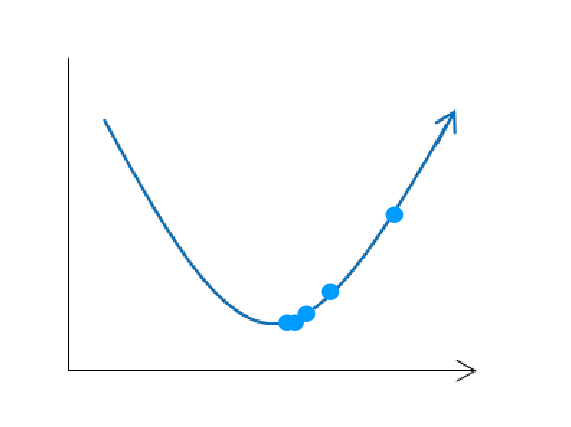
Gradient descent works by randomly selecting a point, calculating the partial derivatives to get the gradient (the vector of all partial derivatives). The gradient will always point in the direction of maximum ascent. Since we want to minimize our function all we need to do is move in the opposite direction of the gradient. We will move along this path some small amount proportional to the negative gradient, this amount is called the learning rate. We then repeat the above steps with our new point (instead of a random one).
If we choose an appropriate learning rate we should get to a point where after many iterations we either arrive at the minimum or at every step we have not made a ‘significant’ improvement, so we stop our algorithm and produce a solution.
If we choose a learning rate that is too large however, we might end up with something like what we see below.

Since our learning rate was large we completely passed over the minimum point and our solution fails to converge at the minimum.
There are a few different ways we can decide on our learning rate, the two most common choices are to set the learning rate to some fixed amount, or to decrease the size of the learning rate at each step. Typically using a fixed learning rate will be fine because as we approach the minimum our slope decreases and so our step size will naturally decrease.
Finding a cost function’s minimum can be pretty straight forward for convex functions, such as in the case of the linear regression cost function.

No matter where you start along the surface you will end up at the global minimum using gradient descent.
However some functions have minima. Below is an example of a function with one local minimum in addition to its global minimum.

If we use gradient descent, depending on where we start, we may end up thinking that the local minimum is the true minimum of our function. Even worse if we get really unlucky we could land directly on the saddle point, where the derivative is zero, and gradient descent algorithm will prematurely stop.
For computational simplicity it is common to choose cost functions that are convex so that we don’t deal with the issues.